astreamline= acceleration along a streamline [m/s2]
C = discharge coefficient [unitless]
dƒ = primary contraction diameter during actual flow conditions [m]
Dƒ = pipe diameter during actual flow conditions [m]
ƒshear = fluid shear stress [N/m2]
glocal = local gravitational constant [m/s2]
Helevation = elevation above a datum [m]
Pflow = pressure at flow conditions [Pa]
ΔP = pressure differential [Pa]
qmass = mass flowrate at flowing conditions [kg/s]
qvolume = volumetric flowrate at flowing conditions [m3/s]
Y1 = adiabatic expansion factor [unitless]
ρflow= density at flowing conditions [kg/m3]
The quantification of volumetric or mass flow is one of the most difficult measurements to make — even in a well-characterized fluid. This is made more difficult in a demanding environment, such as a cryogenic fluid. The value determined often has great impact on the work being conducted, particularly in liquid propulsion systems. Commonly used instrumentation measurement techniques include the use of differential producers, such as Venturi-, flow nozzle-, and orifice plate-type devices. The performance of these instruments in actual application in transient multiphase cryogenic systems is typically one to two orders of magnitude poorer than manufacturer specifications. And while differential producer-based systems are commonly applied in such environments, they have inherent theoretical limitations that affect their accuracy, reliability, and repeatability. These limitations are discussed hereafter. Volumetric & Mass FlowFundamentally, volumetric flow or mass flow is the amount of volume or mass, flowing through some sort of channel per unit time. The channel may be open (trough) or closed (pipe), but must allow for the passage of fluid. (Equation 1)
Conceptually volumetric flow and mass flow are simple. However, a closer look at each term shows the difficulty of making a valid measurement.
The cross-sectional area of a pipe tends to be the easiest to account for. The associated errors directly relate to the error in the physical measurement of diameter. Care must be taken to account for changes in the cross-sectional area (or diameter). These may include: thermal contraction, caking or debris accumulation, etc. Secondary effects, such as pressure bulging and pipe eccentricity or concentricity, and the effect of roughness changes with time on the velocity profile (Reynolds number) must also be considered to further improve the measurement.


With Y1 as the adiabatic expansion factor, C as the discharge coefficient and df, Df as the primary contraction diameter and pipe diameter during actual flow conditions. These parameters are described in the following section.
Correction Terms
It is important to describe the various correction terms that play a role in Equation 4. To begin with, the discharge coefficient, C, is a lump-sum correction term that provides the "fix" from the theoretical system to the real system. The discharge coefficient may be calculated depending on the type of flowmeter. These vary in error from about 0.4 for an uncalibrated meter to 2 percent [2], depending on meter type. This error is a systematic error and is in addition to any other errors (systematic or random). The discharge coefficient can also be determined through calibration. This must be done in the exact same system and under the exact same conditions and environments that the sensor will be used. Rarely is this accomplished, but instead manufacturer calibrations are taken from "like" systems. Particularly in cryogenic devices, water is used as a calibration fluid. The discharge coefficient for the meters shown in Figure 1 range from 0.6 for the orifice to 0.995 for the Venturi and nozzle. The abrupt change in streamlines, however, results in substantial additional pressure loss for the nozzle and orifice. This sometimes results in the unwanted flashing to a vapor.

The term Y1 describes the gas expansion of the fluid, which can be an empirically derived function or theoretically determined, such as the adiabatic gas expansion factor. For an assumption of purely liquid flow this becomes unity. This is even assumed in cryogenics at or near their boiling points. The slightest multiphase component can seriously undermine this approximation. Normally this term is ignored, and its effects are hidden in the discharge coefficient. The fallaciousness is that when the discharge coefficient is used to calibrate the system, it is assumed that the system is corrected over a range of environmental conditions. In reality, the gas expansion term may vary depending on the amount of vapor present this may continuously fluctuate with slight differences in environmental conditions from calibration.
As mentioned earlier, the physical diameters are df, Df. These are the respective bore and pipe diameters. They describe the expansion and contraction of the flow container (pipe and meter bore) due to pressure and temperature effects. These are particularly critical in cryogenic systems where extreme low temperatures cause considerable material contraction. These coefficients require accurate pressure and temperature information in addition to an accurate understanding of the fluid interaction with the pipe material. There is also the added assumption that the temperature and pressure in the pipe or bore match closely with the pressure or temperature sensor location (see below).
The pressure differential, ΔP, is only as valid as the pressure measuring device. Since the mass flow or volumetric flow is determined from a differential pressure measurement it is critical that this value be well characterized. Ideally, the pressure sensors are properly calibrated and corrected for environmental effects such as temperature. Additional factors may include frequency response effects related to the response of the pressure sensor and mounting offset usage (sense lines) [6].
Lastly, rfluid, the fluid density term, describes the density of the fluid. There are numerous tabulated values for various fluids under many thermodynamic conditions. These were developed from highly accurate equations of state that accurately define the density the fluids properties from temperature and pressure measurements. The use of flow computers to compute the necessary fluid properties using these state equations is becoming increasingly more popular. These methods, however, are not foolproof. Small errors in the measures of pressure and temperature can adversely affect the density generated.
Temperature probes may be located near the differential device and can provide a localized measure of temperature. Unfortunately at the temperatures considered here they tend to behave as heat pipes, coupling the environment outside the pipe into the fluid. They also tend to have low response times, on order of seconds [7], leading to latencies under non-steady state conditions. Pressure sensors, on the other hand, tend to average over large fluid volumes, thereby under-representing jumps or steps in the fluid state under a transient condition.
For flow conditions where the thermodynamic state is well defined the computation-based approach to density enables a high-accuracy flow measurement. Careful consideration must be made when the fluid state is not well understood or transient and/or multiphase conditions limit the validity of the supporting instrumentation.
In addition to the theoretical limitations inherent to these devices, differential flowmeters have been tested in characterized in multiphase transient environments. Errors increase dramatically for any deviation from single-phase and steady-state flow conditions. Work at NASA’s Johnson Space Center on flow sensor feasibility has shown errors in using Venturi-type devices ranging from 10 percent to 40 percent in transient and multiphase cryogenic flows [8].
More often than not Web- or pamphlet-based flow discussions begin with Bernoulli’s equation to derive the necessary working equations. Before Bernoulli’s equation can be applied to a fluid environment critical concessions have to be made that limit the applicability and accuracy of differential flowmeters. Clearly the critical measurement component lacking is understanding the thermodynamic and density conditions of the fluid. While quite acceptable in more benign fluid environments, differential-pressure flow devices are greatly limited in transient cryogenic fluid applications. The user must take care when using such devices in these difficult flow conditions.
Valentin Korman, Ph.D., of Madison Research CorporationWFI, has 10 years of sensors, instrumentation, and testing research development experience. Recent efforts have focused on evaluation and development of cryogenic flowmeter technologies. Dr. Korman can be reached at [email protected] or (256) 544-4625
John Wiley, of NASA Marshall Space Flight Center, has 17 years test experience with cryogenic propulsion systems, as well as research and development of advanced sensors for propulsion applications and experience with data validation and electrical and mechanical systems.
Richard W. Miller, Ph.D., of R.W. Miller & Associates, Inc., is a consultant to industry in various flow system and flowmetering areas. He was previously senior consultant with the Foxboro Company and serves, or has served, on many standards and technical committees, both nationally and internationally. Dr. Miller is the author of the "Flow Measurement Engineering Handbook" (McGraw Hill).
References
1. R. M. Olson, Essentials of Engineering Fluid Dynamics, 2nd Edition, International Textbook Co., 1967.
2. Richard W. Miller, Flow Measurement Engineering Handbook, 3rd Edition, McGraw-Hill, 1996.
3. H. M. Roder and L. A. Weber, Thermophysical Properties-ASRDI Oxygen Technology Survey, Volume 1, NASA SP-3071, 1972.
4. D. R. Lide, CRC Handbook of Chemistry and Physics, 71st Edition, CRC Press, 1991.
5. Korman V., Gregory D. A., and Wiley J. T. Mass Flow Measurement in a Cryogenic System using a Fiber Optics-Based Dispersion Sensor, Propulsion Measurement Sensor Development Workshop, Huntsville, AL May 2003. Proceedings.
6. Wiley J. T., Korman V., Vitarius P. T., and Gregory D. A., Acoustic Wave Propagation in Pressure Sense Lines, Presented at 39th AIAA/ASME/SAE/ASEE Joint Propulsion Conference, 2003, Proceedings.
7. Nanmac, Comparison of Temperature Sensor Response Times,
www.nanmac.com.
8. R.S. Baird, Flowmeter Evaluation for On-orbit Operations, NASA TM-100465, Johnson Space Center, August 1988.